(working title: Identifying symbol-tokens by measuring pixel-correlations within documents)

So since there are only black and white pixels, i runs from 1 to n=2, and b the base is 2 by convention. P just means the Probability of appearance of the corresponding color xi, which is easily calculated by dividing the absolute number of black rpt. white pixels through the total number of pixels overall.
There's an interesting trick here: whenever the number of black and white pixels are equal, the maximum amount of information for the amount of pixels given is conveyed. Whenever there are more white than black or more black than white pixels, the information content get's less and less, due some kind of unbalance. This is pure mathematics and can be seen in the following chart:

The maximum of information is in the middle, when black equals white (Probability of Black plotted horizontal). The more both are out of balance, the less information is contained in the sequence considered. Think of it as in the following exemplification: when something happens more often, it get's more and more expectable, therefore giving you less information (that's the log-part of the Formula), when on the other hand something get's rarer and rarer, it gives you more information when it happens! And as you can see in the above illustration, the gain on one color's information-value cannot compensate for the loss of the other.
The total loss in information due to this unbalance is called redundancy.
This is not the "Shannon Paradoxon" - these were just the basics!
Intermezzo
If we look onto an alphabet consisting of more than two letters - e.g. our latin alphabet - there's the same principle: if all occurrence probabilities are equal, the most information possible with this alphabet is transmitted. As soon as the probabilities get unbalanced, the total amount of information gets reduced. Again, some letters contain more information, because they occur more seldom; but this cannot make up for its smaller contribution to the total information sum due to its sparsity.
 |
| unbalanced distribution - information per letter: 4.2297 bit |
 |
| uniformly distributed - information per letter: 4.7004 bit |
The Shannon Paradoxon...
Shannon-Information Theorie provides a simple formula for calculating the information-content of an information probe. All you need to identify is your alphabet and additionally make sure, that the single letters contained within the alphabet are independent in their appearance probability...
But there is a loophole: in reality letters are not independent but interdependent - that's called correlation (a kind of redundancy as we will see later...).
Put in one sentence: "You cannot measure the information of a given pixel stream, by just looking at it on pixel level."
Yes, that sounds like a contradiction to the definition given above, but i will (try to) get clearer in a minute...
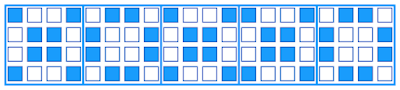
Look at the following sequence consisting of 80 pixels:
You can count all of them - if you want - but I will assure you that there are 40 black ones and 40 white ones. So according to Shannons Formula, given above, we get 80 bits of Information, because when both colors are equal we get the maximum of information per pixel, which is one bit.
But now look at the following picture:
What happened? - I combined every 16 pixels and rearranged them in the form of a 4x4 quad. Now the human eye can recognize, that our initial stream consists of 5 blocks making up 5 symbols (XOXXO) of which there are only 2 different kinds: X and O.
That's what normally a compression algorithm does: looking for patterns that allow the sequence to be represented by less space, subsequently holding less information. Less information means more redundancy and notice that this kind of redundancy is of a different "smell"... (sometimes it is called correlation between the pixels of one grouping - i you will, you can think of it as the strength of the capability of the letters to be autocompleted to the whole letter on pixel-level, when some pixels are given..).
To summarize: first at pixel level we thought we have 80 bits of information. After looking at the "bigger picture" we recognized, that we only have about 5 bits (because every symbol gives approximately 1 bit: H=2/5*log2(5/2)+3/5*log2(5/3)=0.97...).
...and how to solve it
So the solution is, to look at your information on different levels, or as I call them: at different window sizes.
Look at the following letter square made up from 25 letters of the latin alphabet:

The letters are given by a 40x40 pixel quad. We first examine it on pixel-sequence-level. Then we increase the 1 pixel window size, step by step, until we reach the whole document.

In the first step there are 1600 pixels, 706 of them black, 894 white - believe me or count them. According to Shannon we have 0.990017851983 bits per pixel making up for 1584 bits of information altogether. But there was this thing called redundancy. Remember: you only can detect redundancy when increasing you pixel window size (and so make the correlation between them visible). So in the next step we examine the data probe by slicing it into 2x2 quad patches. From the theoretically 2^4=16 possible patches, only 14 occur, - they are given here together with their frequencies:

The information amount per 2x2 patch is 3.2266832597 bit. So, why isn't it 4 bit? After all there are 4 pixels here! Answer: there's a discount because of the unbalanced occurrence statistic! All together this sums up to 1291 bits of information. Notice, that the number is going down rapidly...
So in the next step we examine a patch size of 4x4, because we don't like to allow a 'gliding' patch, that stops at every position, but a proper slicing of the 40x40 field into even patches i.e. divisors of 40. We don't do overlapping patches here, because we don't want to count information "multiple" times...
The information amount per 4x4 patch is 5.59391900518 bit. Overall information amount: 559 bits.
If we continue with the same rhythm we get the following patches/frequencies/information amounts:
5x5 information per patch: 6 bits, information overall: 384 bits
With 8x8 patches we finally get what I call the "intended level of transfer": our latin alphabet:
8x8 ipp: 4.64385618977 = log2(25) bits, overall: 116 bits
With bigger patches we get the following results:
10x10 ipp: 4 bit, overal: 64 bits
20x20 ipp: 2 bit, overall: 8 bit
In summary one can see, that with increasing patch sizes, the information per patch (red) goes down, because the number of different patches gets less and less.
The information per pixel (blue) has a maximum, but unfortunately with a smaller Patch Size than 8.
Let's reconsider: we are in need of a formula, that get's us an optimum for the 8x8 patches level of observation. Additional we have to overcome the fact, that our setting is biassed, because of the very restricted area, not allowing for many different Patches of the bigger kind.
 |
| Information per pixel (blue) - Information per patch (red) |
It seems that something is missing here: we are in need of a counterpart, that compensates, so that we get some kind of equilibrium "in the middle" - hopefully at patchsize 8x8...
A new Perspective
Imagine stacking all resulting e.g. 2x2 patches on top of each other - so that every pixel gets positioned over its corresponding counterpart along all of the other patches:

The different Patches constitute our resulting Alphabet. The Information delivered by one Letter of this Alphabet can be calculated on four different levels of abstraction in four different ways:
The first two methods are looking on the patches on pixel level.
R0 - Pixel level, straight
Every Patch consists of four pixels, every pixel represents potentially 1 bit, so altogether we have 4 bit.
R1 - Pixel level, Shannon
Every Pixel Position can hold a white or black Pixel - we must therefor calculate the Information Content of every Pixel Position by applying Shannons Formula (s.a.); particularly we must count the white and black pixel frequencies by vertically going through all Patches; e.g. upper left Pixel Position: frequency for white: 192, frequency for black: 208 - this yields an over information for this Pixel Position of: 0,99885 bit (the other three values are calculated accordingly yielding a total Information of 3.8953 bit per Patch).
The third and forth method are looking at the patches on patch level.
R2 - Patch level, Shannon
Since each of the 15 Patches has given its occurrence frequency, it's straight forward to calculate the median information of a Patch according to Shannons Formula on Patch level. This results in 3.2266 bit.
R3 - Patch level, optimal
If all Patches would occur with equal probability, then the information content would be even more than this, it could be calculated by log2(16) = 4 bit.
This overview gives all Formulas for the 4 levels of abstraction:

Choosing a Metric
When plotting all 4 Information Contents, we get the following Chart:


We choose two measurements:
Redundancy of the Patch Alphabet
According to Shannons Formula the Difference between R2 and R3 is called the redundancy of the Patch - we calculate the relative redundancy: 1-R2/R3.
Correlation of the Pixels grouped within the Patches
We cannot calculate this Correlation directly: therefore we use the difference of the Information maximally possible for one Patch (R2) and the Information that is differentiated "vertically" from the pixels perspective (R1) - since we calculate again the relative correlation we use a differential quotient: (R1-R2)/(R0-R2).
As a result we get the following wonderful diagram, that shows how combining minimal Redundancy with minimal Correlation yields an Optimum for Patch Size 8:

So, why does it work?
At first we look at the relative Redundancy of the Alphabet. When at Pixel Level, in an ordinary Text Document, the white Pixels outweigh the black ones, by a factor of 4 (if not more) approximately. This means the relative Redundancy is in the Area of 25-30%. When Patches grow bigger, this imbalance gets distributed and capsuled in Combinations of black and white Pixels, that are imbalanced within the Patch, but from the outside Patch Frequencies are balanced. In case of the latin Alphabet, the imbalance (as mentioned above: 4.2297/4.7004) results in a relative Redundancy of ~ 10%. This gets better and better, as the Patch Size grows, because the resulting Combinations of Letters and Letter Fragments are so unique, that every single Patch occurs only once, and therefor by definition relative Redundancy goes to zero.
So, for getting an optimum, we are in need of a second factor: The Correlation of the Pixels constituting the Patch. The crucial Point, when looking at a Patch on Pixel Level, is that it suggests, that there is much more information contained, than afterwards emerges on Patch Level. So we have to propagate downwards the information contained in one Patch and distribute it over the existing Pixels. On Patch Level, the Information of one Patch is log2(Size of Patch Alphabet). So one thing is clear: not every Pixel Position can unfold its full potential to differentiate (that's what information is) to the full extent of 1 bit. (this would be the case, if in the half of Patches on this Pixel Position there would be a black Pixel an in the other half a white one... - 0 bit would be the case, when the color for a particular Pixel Position would be the same for all Patches black or white...). The metric's goal is, to minimize the difference between the Sum of all Pixels' local Information Contents and the Patch Information. (btw. this difference can be called the Autocompletion-Capability of any Patch, in the sense, that you can derive the full Patch, from knowing only few Pixels - Why don't we want Autocompletion? - That's another Question, we'll answer in the future). So all Pixel-local Information Contents should be pushed down to around log2(Size of Patch Alphabet)/(Number of Pixels per Patch) on average. But how to distribute the available Information over the existing Pixels? There are two Possibilities: even or with cumulations. When choosing even, the human perception apparatus gets a problem; so we choose the second. Human Perception likes to discover Patterns, which are Redundancies, Repetitions of the same. These are used as Positioning Markers, to differentiate the Position of each Letter. So the best Patch Alphabet consists of one Set of Pixel Positions, which are identical in nearly every Patch, constituting the Positional Information; and a second Set consisting of Pixel Positions which differ greatly among the Patches, bearing the Differentiating Information. This is what is what is captured by the second metric.
Remark: This second factor (or rather the Marker regions) is btw. also the reason, that the first delivers a suboptimal result, when Patch Size is below (latin) Letter Size: there are many equal Patches, that are (Sub-)Parts of the Marker Regions making for a great unbalancedness...
Another Remark: Vice versa, a great Unbalancedness (bad first factor) could make for a good (low) Correlation, because of many same Patches, that reduce the Pixel-local Information Content and therefor must be ruled out.
So one can see, that both factors are real Antagonists and make great ingredients for a combined Metric.
Next Steps
Notice that there's still a problem lurking around. We have chosen our slicing so perfectly, that by a miraculous coincidence all letters are met with offset zero! (when patch size equals letter size, 8x8). So, what can we do to overcome this challenge?
Remember the last blog about "Positional Information"? That's exactly what we need to give an even better version of the algorithm that even works for arbitrary offsets. We will iterate through all possible offsets and find the right one by giving a third parameter, that gets optimal when all letters come exactly over each other when patches are stacked.
Remember the last blog about "Positional Information"? That's exactly what we need to give an even better version of the algorithm that even works for arbitrary offsets. We will iterate through all possible offsets and find the right one by giving a third parameter, that gets optimal when all letters come exactly over each other when patches are stacked.
This third parameter will be the relative information contained in a patch measured via it's pixels horizontally! That means how many black/white pixels are contained in the patch, and how many information is therefore contained in one pixel at average (s. first picture of this blog) according to Shannon's Formula. This will then be averaged over all patches.
Additionally we should make sure, that the Formula works also for settings with bigger Documents, consisting of many more than 25 Letters.
Download the Code
-> here
%matplotlib inline
import matplotlib.pyplot as plt
from matplotlib.ticker import NullFormatter
import numpy as np
from sklearn.feature_extraction.image import extract_patches
from math import log
import pandas as pd


### 7x7 - alphabet
Z=np.array([(0, 0, 1, 1, 1, 0, 0, 0, 1, 1, 0, 1, 1, 0, 1, 1, 0, 0, 0, 1, 1, 1, 1, 0, 0, 0, 1, 1, 1, 1, 1, 1, 1, 1, 1, 1, 1, 0, 0, 0, 1, 1, 1, 1, 0, 0, 0, 1, 1),
(1, 1, 1, 1, 1, 1, 0, 1, 1, 0, 0, 0, 1, 1, 1, 1, 0, 0, 0, 1, 1, 1, 1, 1, 1, 1, 1, 0, 1, 1, 0, 0, 0, 1, 1, 1, 1, 0, 0, 0, 1, 1, 1, 1, 1, 1, 1, 1, 0),
(0, 0, 1, 1, 1, 1, 0, 0, 1, 1, 0, 0, 1, 1, 1, 1, 0, 0, 0, 0, 0, 1, 1, 0, 0, 0, 0, 0, 1, 1, 0, 0, 0, 0, 0, 0, 1, 1, 0, 0, 1, 1, 0, 0, 1, 1, 1, 1, 0),
(1, 1, 1, 1, 1, 0, 0, 1, 1, 0, 0, 1, 1, 0, 1, 1, 0, 0, 0, 1, 1, 1, 1, 0, 0, 0, 1, 1, 1, 1, 0, 0, 0, 1, 1, 1, 1, 0, 0, 1, 1, 0, 1, 1, 1, 1, 1, 0, 0),
(1, 1, 1, 1, 1, 1, 1, 1, 1, 0, 0, 0, 0, 0, 1, 1, 0, 0, 0, 0, 0, 1, 1, 1, 1, 1, 1, 0, 1, 1, 0, 0, 0, 0, 0, 1, 1, 0, 0, 0, 0, 0, 1, 1, 1, 1, 1, 1, 1),
(1, 1, 1, 1, 1, 1, 1, 1, 1, 0, 0, 0, 0, 0, 1, 1, 0, 0, 0, 0, 0, 1, 1, 1, 1, 1, 1, 0, 1, 1, 0, 0, 0, 0, 0, 1, 1, 0, 0, 0, 0, 0, 1, 1, 0, 0, 0, 0, 0),
(0, 0, 1, 1, 1, 1, 1, 0, 1, 1, 0, 0, 0, 0, 1, 1, 0, 0, 0, 0, 0, 1, 1, 0, 0, 1, 1, 1, 1, 1, 0, 0, 0, 1, 1, 0, 1, 1, 0, 0, 1, 1, 0, 0, 1, 1, 1, 1, 1),
(1, 1, 0, 0, 0, 1, 1, 1, 1, 0, 0, 0, 1, 1, 1, 1, 0, 0, 0, 1, 1, 1, 1, 1, 1, 1, 1, 1, 1, 1, 0, 0, 0, 1, 1, 1, 1, 0, 0, 0, 1, 1, 1, 1, 0, 0, 0, 1, 1),
(1, 1, 1, 1, 1, 1, 0, 0, 0, 1, 1, 0, 0, 0, 0, 0, 1, 1, 0, 0, 0, 0, 0, 1, 1, 0, 0, 0, 0, 0, 1, 1, 0, 0, 0, 0, 0, 1, 1, 0, 0, 0, 1, 1, 1, 1, 1, 1, 0),
(0, 0, 0, 0, 0, 1, 1, 0, 0, 0, 0, 0, 1, 1, 0, 0, 0, 0, 0, 1, 1, 0, 0, 0, 0, 0, 1, 1, 0, 0, 0, 0, 0, 1, 1, 1, 1, 0, 0, 0, 1, 1, 0, 1, 1, 1, 1, 1, 0),
(1, 1, 0, 0, 0, 1, 1, 1, 1, 0, 0, 1, 1, 0, 1, 1, 0, 1, 1, 0, 0, 1, 1, 1, 1, 0, 0, 0, 1, 1, 1, 1, 1, 0, 0, 1, 1, 0, 1, 1, 1, 0, 1, 1, 0, 0, 1, 1, 1),
(1, 1, 0, 0, 0, 0, 0, 1, 1, 0, 0, 0, 0, 0, 1, 1, 0, 0, 0, 0, 0, 1, 1, 0, 0, 0, 0, 0, 1, 1, 0, 0, 0, 0, 0, 1, 1, 0, 0, 0, 0, 0, 1, 1, 1, 1, 1, 1, 1),
(1, 1, 0, 0, 0, 1, 1, 1, 1, 1, 0, 1, 1, 1, 1, 1, 1, 1, 1, 1, 1, 1, 1, 1, 1, 1, 1, 1, 1, 1, 0, 1, 0, 1, 1, 1, 1, 0, 0, 0, 1, 1, 1, 1, 0, 0, 0, 1, 1),
(1, 1, 0, 0, 0, 1, 1, 1, 1, 1, 0, 0, 1, 1, 1, 1, 1, 1, 0, 1, 1, 1, 1, 1, 1, 1, 1, 1, 1, 1, 0, 1, 1, 1, 1, 1, 1, 0, 0, 1, 1, 1, 1, 1, 0, 0, 0, 1, 1),
(0, 1, 1, 1, 1, 1, 0, 1, 1, 0, 0, 0, 1, 1, 1, 1, 0, 0, 0, 1, 1, 1, 1, 0, 0, 0, 1, 1, 1, 1, 0, 0, 0, 1, 1, 1, 1, 0, 0, 0, 1, 1, 0, 1, 1, 1, 1, 1, 0),
(1, 1, 1, 1, 1, 1, 0, 1, 1, 0, 0, 0, 1, 1, 1, 1, 0, 0, 0, 1, 1, 1, 1, 0, 0, 0, 1, 1, 1, 1, 1, 1, 1, 1, 0, 1, 1, 0, 0, 0, 0, 0, 1, 1, 0, 0, 0, 0, 0),
(0, 1, 1, 1, 1, 1, 0, 1, 1, 0, 0, 0, 1, 1, 1, 1, 0, 0, 0, 1, 1, 1, 1, 0, 0, 0, 1, 1, 1, 1, 0, 1, 1, 1, 1, 1, 1, 0, 0, 1, 1, 0, 0, 1, 1, 1, 1, 0, 1),
(1, 1, 1, 1, 1, 1, 0, 1, 1, 0, 0, 0, 1, 1, 1, 1, 0, 0, 0, 1, 1, 1, 1, 0, 0, 1, 1, 1, 1, 1, 1, 1, 1, 0, 0, 1, 1, 0, 1, 1, 1, 0, 1, 1, 0, 0, 1, 1, 1),
(0, 1, 1, 1, 1, 0, 0, 1, 1, 0, 0, 1, 1, 0, 1, 1, 0, 0, 0, 0, 0, 0, 1, 1, 1, 1, 1, 0, 0, 0, 0, 0, 0, 1, 1, 1, 1, 0, 0, 0, 1, 1, 0, 1, 1, 1, 1, 1, 0),
(1, 1, 1, 1, 1, 1, 0, 0, 0, 1, 1, 0, 0, 0, 0, 0, 1, 1, 0, 0, 0, 0, 0, 1, 1, 0, 0, 0, 0, 0, 1, 1, 0, 0, 0, 0, 0, 1, 1, 0, 0, 0, 0, 0, 1, 1, 0, 0, 0),
(1, 1, 0, 0, 0, 1, 1, 1, 1, 0, 0, 0, 1, 1, 1, 1, 0, 0, 0, 1, 1, 1, 1, 0, 0, 0, 1, 1, 1, 1, 0, 0, 0, 1, 1, 1, 1, 0, 0, 0, 1, 1, 0, 1, 1, 1, 1, 1, 0),
(1, 1, 0, 0, 0, 1, 1, 1, 1, 0, 0, 0, 1, 1, 1, 1, 0, 0, 0, 1, 1, 1, 1, 1, 0, 1, 1, 1, 0, 1, 1, 1, 1, 1, 0, 0, 0, 1, 1, 1, 0, 0, 0, 0, 0, 1, 0, 0, 0),
(1, 1, 0, 0, 0, 1, 1, 1, 1, 0, 0, 0, 1, 1, 1, 1, 0, 1, 0, 1, 1, 1, 1, 1, 1, 1, 1, 1, 1, 1, 1, 1, 1, 1, 1, 1, 1, 1, 0, 1, 1, 1, 1, 1, 0, 0, 0, 1, 1),
(1, 1, 0, 0, 0, 1, 1, 1, 1, 1, 0, 1, 1, 1, 0, 1, 1, 1, 1, 1, 0, 0, 0, 1, 1, 1, 0, 0, 0, 1, 1, 1, 1, 1, 0, 1, 1, 1, 0, 1, 1, 1, 1, 1, 0, 0, 0, 1, 1),
(1, 1, 0, 0, 1, 1, 0, 1, 1, 0, 0, 1, 1, 0, 1, 1, 0, 0, 1, 1, 0, 0, 1, 1, 1, 1, 0, 0, 0, 0, 1, 1, 0, 0, 0, 0, 0, 1, 1, 0, 0, 0, 0, 0, 1, 1, 0, 0, 0)])
#25! (1, 1, 1, 1, 1, 1, 1, 0, 0, 0, 0, 1, 1, 1, 0, 0, 0, 1, 1, 1, 0, 0, 0, 1, 1, 1, 0, 0, 0, 1, 1, 1, 0, 0, 0, 1, 1, 1, 0, 0, 0, 0, 1, 1, 1, 1, 1, 1, 1)])

### analyze patch-wise
def calc_patches(m):
    #print (np.concatenate(ba, axis=1).shape)
    patches = extract_patches(ff, (m, m), (m,m)) #,patch_size =(2, 2), extraction_step=(1, 1)) #das waere dann gleitend
    patches = patches.reshape(-1, m*m) #2, 2) # -1 means: automatic!
    all_patches=patches.shape[0]

    cnt_patches=0
    info_patches=0
    ### gliding all_patches=(5*8-(m-1))*(5*8-(m-1))
    vertical_info=np.zeros(m*m)
    fig = plt.figure(figsize=(100,2))

    lista = [ tuple(x) for x in patches ]

    total_patches=len(pd.Series(lista).value_counts())

    for k,g in pd.Series(lista).value_counts().iteritems():
        cnt_patches+=1
        info_patches +=(g/all_patches)*log(1.*all_patches/g,2)
        for x in range(len(k)):
            if(k[x]==1):
                vertical_info[x]+=g
        c=np.reshape(k,(m,m))
        ax = fig.add_subplot(1,total_patches,cnt_patches)
        ax.imshow(c, interpolation='none', cmap=plt.cm.gray_r)
    print("\n")
    print("Frame-Window-Size -->",m,"x",m,"(=",m*m," Pixels)")
    print("Number of Patches: ",lpr*ppr/m,"x",lpr*ppr/m,"=",all_patches) #?
    plt.show()

    print("number of occurring DIFFERENT patches:",total_patches)
    print("number of THEORETICALLY possible DIFFERENT patches: 2^",m*m,"=",2**(m*m))

    info_pixel=0
    for i in range(len(vertical_info)):
        if(vertical_info[i]!=0 and all_patches!=vertical_info[i]):
            info_pixel+=(vertical_info[i]/all_patches)*log(1.*all_patches/vertical_info[i],2)+(1-(vertical_info[i]/all_patches))*log(1.*all_patches/(all_patches-vertical_info[i]),2)
    print("\n")
    print("R0: Number of Pixels in Patch (bit)",m*m)
    print("R1: Vertical Information per Pixel accumulated over Patch",info_pixel)
    print("R2: average Information per Patch (weighted by occurrenes)",info_patches)
    print("R3: average Information per Patch (equiprobable patches)",log(total_patches,2))
    print("--------------------------------------------------")
    relative_alphabet_redundancy = 1-(info_patches/log(total_patches,2))
    relative_alphabet_correlation = (info_pixel-info_patches)/(m*m-info_patches)
    print("Relative Alphabet Redundancy: 1-R2/R3", relative_alphabet_redundancy)
    print("Relative Alphabet Correlation: (R1-R2)/(R0-R2)", relative_alphabet_correlation)
    return(relative_alphabet_redundancy, relative_alphabet_correlation)
    #trick, 2var behind return( 1-(info_patches/log(total_patchescnt_patches,2)), (info_pixel-info_patches)/(m*m-info_patches))


b =[]
lpr=5 ### letter ppr row
ppro=7 ### pixel ppr row (ori, w/o padding)
pad=1 ### padding
ppr=ppro+pad ### pixel ppr row (w/ padding)

### build up letters
fig = plt.figure(figsize=(10,2)) #plt.figure(figsize=(1,1))
for a in range(len(Z)):
    ax = fig.add_subplot(1,len(Z),a+1)
    c=np.pad(Z[a].reshape(ppro,ppro), ((0,pad),(0,pad)), mode='constant') ##auf"patchen" auf 9x9 bzw 8x8...
    b.append(np.array(c))
    ax.imshow(c, interpolation='none', cmap=plt.cm.gray_r) #binary, nearest, bicubic, bilinear
    ax.axes.get_xaxis().set_major_formatter(NullFormatter())
    ax.axes.get_yaxis().set_major_formatter(NullFormatter())
    plt.xticks(np.arange(-0.5, 3.5, 1.))
    plt.yticks(np.arange(-0.5, 3.5, 1.)) ##([])
    plt.grid(True)
print("intended Alphabet")
plt.show()

### form square
ba = np.array(b)
cc=ba.reshape(lpr,lpr,ppr,ppr)
dd=[]
for i in range(lpr):
    dd.append(np.concatenate(cc[i], axis=1))
ee=np.stack(dd)
ff=ee.reshape(lpr*ppr,lpr*ppr)

### show 'document'
print("given Document")
plt.imshow(ff, cmap=plt.cm.binary, interpolation='none')
plt.show()

### calc patches
x = []
y = []
y2= []
y3= []
for a in (2,4,5,8,10,20): #divisors of 40
    x.append(a)
    a1, a2 = calc_patches(a)
    y.append(a1)
    y2.append(a2)
    y3.append((a1+a2)/2.0) #why arithmetic?
plt.plot(x,y,label="Redundancy in Patch Alphabet")
plt.plot(x,y2,label="Pixel Correlation in Patches")
plt.plot(x,y3,label="Combined Average (arithm.))")
plt.legend(loc="upper right")
plt.annotate('minimum',
            xy=(8, 0.3),  # theta, radius
            xytext=(0.6, 0.2),    # fraction, fraction
            textcoords='figure fraction',
            arrowprops=dict(facecolor='black', shrink=0.05),
            horizontalalignment='left',
            verticalalignment='bottom')
plt.show()
References
Keine Kommentare:
Kommentar veröffentlichen